定义:
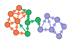
k均值聚类算法(k-means clustering algorithm)是一种迭代求解的聚类分析算法,其步骤是,预将数据分为K组,则随机选取K个对象作为初始的聚类中心,然后计算每个对象与各个种子聚类中心之间的距离,把每个对象分配给距离它最近的聚类中心。聚类中心以及分配给它们的对象就代表一个聚类。每分配一个样本,聚类的聚类中心会根据聚类中现有的对象被重新计算。这个过程将不断重复直到满足某个终止条件。终止条件可以是没有(或最小数目)对象被重新分配给不同的聚类,没有(或最小数目)聚类中心再发生变化,误差平方和局部最小。
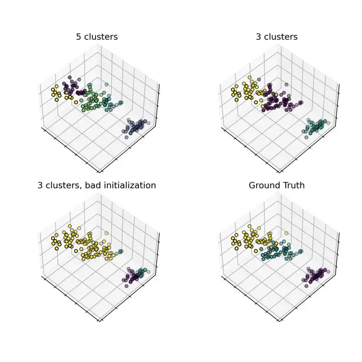
K均值聚类算法,示例一
"""=========================================================K-means Clustering=========================================================The plots display firstly what a K-means algorithm would yieldusing three clusters. It is then shown what the effect of a badinitialization is on the classification process:By setting n_init to only 1 (default is 10), the amount oftimes that the algorithm will be run with different centroidseeds is reduced.The next plot displays what using eight clusters would deliverand finally the ground truth."""import numpy as npimport matplotlib.pyplot as pltimport mpl_toolkits.mplot3d from sklearn.cluster import KMeansfrom sklearn import datasets#=================iris = datasets.load_iris();X = iris.data;y = iris.target;fig = plt.figure(figsize=(9, 7));plt.subplots_adjust(left=None, bottom=None, right=None, top=None, wspace=0.0, hspace=0.15);#=================estimators = [
    ("k_means_iris_5", KMeans(n_clusters=5)),
    ("k_means_iris_3", KMeans(n_clusters=3)),
    ("k_means_iris_bad_init", KMeans(n_clusters=3, n_init=1, init="random")) ];fignum = 1;titles = ["5 clusters", "3 clusters", "3 clusters, bad initialization"];for name, est in estimators:
    ax = fig.add_subplot(2,2,fignum, projection="3d", elev=48, azim=134);

    est.fit(X);
    labels = est.labels_;
    ax.scatter(X[:, 3], X[:, 0], X[:, 2], c=labels.astype(float), edgecolor="k");

    ax.w_xaxis.set_ticklabels([]);
    ax.w_yaxis.set_ticklabels([]);
    ax.w_zaxis.set_ticklabels([]);
    ax.set_title(titles[fignum -1]);
    fignum = fignum + 1;#=================# Plot the ground truthax = fig.add_subplot(224, projection="3d", elev=48, azim=134);# Reorder the labels to have colors matching the cluster resultsy = np.choose(y, [0,1,2]).astype(float);ax.scatter(X[:, 3], X[:, 0], X[:, 2], c=y, edgecolor="black");ax.w_xaxis.set_ticklabels([]);ax.w_yaxis.set_ticklabels([]);ax.w_zaxis.set_ticklabels([]);ax.set_title("Ground Truth");# saveplt.savefig("plot_cluster_iris.png", dpi=300);
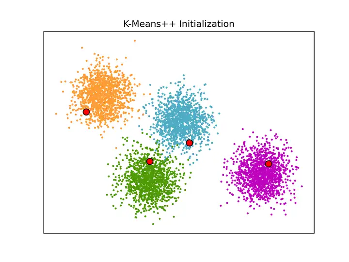
K均值聚类算法,示例二
"""===========================================================An example of K-Means++ initialization===========================================================An example to show the output of the :func:`sklearn.cluster.kmeans_plusplus`function for generating initial seeds for clustering.K-Means++ is used as the default initialization for :ref:`k_means`."""from sklearn.cluster import kmeans_plusplusfrom sklearn.datasets import make_blobsimport matplotlib.pyplot as plt# Generate sample datan_samples = 5000;n_components = 4;X, y_true = make_blobs(n_samples=n_samples, centers=n_components, cluster_std=0.60, random_state=0);X = X[:, ::-1];# Calculate seeds from kmeans++centers_init, indices = kmeans_plusplus(X, n_clusters=4, random_state=0)# Plot init seeds along side sample dataplt.figure(1);colors = ["#4EACC5", "#FF9C34", "#4E9A06", "m"];for k, col in enumerate(colors):
    cluster_data = y_true == k;
    plt.scatter(X[cluster_data, 0], X[cluster_data, 1], c=col, marker=".", s=10);plt.scatter(centers_init[:, 0], centers_init[:, 1], facecolor="red", edgecolor="black", s=70);plt.title("K-Means++ Initialization");plt.xticks([]);plt.yticks([]);plt.savefig("plot_kmeans_plusplus.png", dpi=300);plt.show();
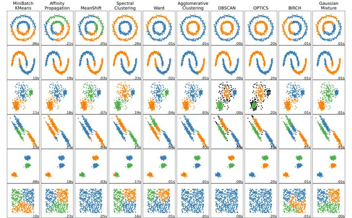
"""=========================================================Comparing different clustering algorithms on toy datasets=========================================================This example shows characteristics of differentclustering algorithms on datasets that are "interesting"but still in 2D. With the exception of the last dataset,the parameters of each of these dataset-algorithm pairshas been tuned to produce good clustering results. Somealgorithms are more sensitive to parameter values thanothers.The last dataset is an example of a 'null' situation forclustering: the data is homogeneous, and there is no goodclustering. For this example, the null dataset uses thesame parameters as the dataset in the row above it, whichrepresents a mismatch in the parameter values and thedata structure.While these examples give some intuition about thealgorithms, this intuition might not apply to very highdimensional data."""import timeimport warningsimport numpy as npimport matplotlib.pyplot as pltfrom sklearn import cluster, datasets, mixturefrom sklearn.neighbors import kneighbors_graphfrom sklearn.preprocessing import StandardScalerfrom itertools import cycle, islicenp.random.seed(0)# ============# Generate datasets. We choose the size big enough to see the scalability# of the algorithms, but not too big to avoid too long running times# ============n_samples = 500noisy_circles = datasets.make_circles(n_samples=n_samples, factor=0.5, noise=0.05)noisy_moons = datasets.make_moons(n_samples=n_samples, noise=0.05)blobs = datasets.make_blobs(n_samples=n_samples, random_state=8)no_structure = np.random.rand(n_samples, 2), None# Anisotropicly distributed datarandom_state = 170X, y = datasets.make_blobs(n_samples=n_samples, random_state=random_state)transformation = [[0.6, -0.6], [-0.4, 0.8]]X_aniso = np.dot(X, transformation)aniso = (X_aniso, y)# blobs with varied variancesvaried = datasets.make_blobs(
    n_samples=n_samples, cluster_std=[1.0, 2.5, 0.5], random_state=random_state)# ============# Set up cluster parameters# ============plt.figure(figsize=(9 * 2 + 3, 13))plt.subplots_adjust(
    left=0.02, right=0.98, bottom=0.001, top=0.95, wspace=0.05, hspace=0.01)plot_num = 1default_base = {
    "quantile": 0.3,
    "eps": 0.3,
    "damping": 0.9,
    "preference": -200,
    "n_neighbors": 3,
    "n_clusters": 3,
    "min_samples": 7,
    "xi": 0.05,
    "min_cluster_size": 0.1,}datasets = [
    (
        noisy_circles,
        {
            "damping": 0.77,
            "preference": -240,
            "quantile": 0.2,
            "n_clusters": 2,
            "min_samples": 7,
            "xi": 0.08,
        },
    ),
    (
        noisy_moons,
        {
            "damping": 0.75,
            "preference": -220,
            "n_clusters": 2,
            "min_samples": 7,
            "xi": 0.1,
        },
    ),
    (
        varied,
        {
            "eps": 0.18,
            "n_neighbors": 2,
            "min_samples": 7,
            "xi": 0.01,
            "min_cluster_size": 0.2,
        },
    ),
    (
        aniso,
        {
            "eps": 0.15,
            "n_neighbors": 2,
            "min_samples": 7,
            "xi": 0.1,
            "min_cluster_size": 0.2,
        },
    ),
    (blobs, {"min_samples": 7, "xi": 0.1, "min_cluster_size": 0.2}),
    (no_structure, {}),]for i_dataset, (dataset, algo_params) in enumerate(datasets):
    # update parameters with dataset-specific values
    params = default_base.copy()
    params.update(algo_params)

    X, y = dataset

    # normalize dataset for easier parameter selection
    X = StandardScaler().fit_transform(X)

    # estimate bandwidth for mean shift
    bandwidth = cluster.estimate_bandwidth(X, quantile=params["quantile"])

    # connectivity matrix for structured Ward
    connectivity = kneighbors_graph(
        X, n_neighbors=params["n_neighbors"], include_self=False
    )
    # make connectivity symmetric
    connectivity = 0.5 * (connectivity + connectivity.T)

    # ============
    # Create cluster objects
    # ============
    ms = cluster.MeanShift(bandwidth=bandwidth, bin_seeding=True)
    two_means = cluster.MiniBatchKMeans(n_clusters=params["n_clusters"])
    ward = cluster.AgglomerativeClustering(
        n_clusters=params["n_clusters"], linkage="ward", connectivity=connectivity
    )
    spectral = cluster.SpectralClustering(
        n_clusters=params["n_clusters"],
        eigen_solver="arpack",
        affinity="nearest_neighbors",
    )
    dbscan = cluster.DBSCAN(eps=params["eps"])
    optics = cluster.OPTICS(
        min_samples=params["min_samples"],
        xi=params["xi"],
        min_cluster_size=params["min_cluster_size"],
    )
    affinity_propagation = cluster.AffinityPropagation(
        damping=params["damping"], preference=params["preference"], random_state=0
    )
    average_linkage = cluster.AgglomerativeClustering(
        linkage="average",
        affinity="cityblock",
        n_clusters=params["n_clusters"],
        connectivity=connectivity,
    )
    birch = cluster.Birch(n_clusters=params["n_clusters"])
    gmm = mixture.GaussianMixture(
        n_components=params["n_clusters"], covariance_type="full"
    )

    clustering_algorithms = (
        ("MiniBatch\nKMeans", two_means),
        ("Affinity\nPropagation", affinity_propagation),
        ("MeanShift", ms),
        ("Spectral\nClustering", spectral),
        ("Ward", ward),
        ("Agglomerative\nClustering", average_linkage),
        ("DBSCAN", dbscan),
        ("OPTICS", optics),
        ("BIRCH", birch),
        ("Gaussian\nMixture", gmm),
    )

    for name, algorithm in clustering_algorithms:
        t0 = time.time()

        # catch warnings related to kneighbors_graph
        with warnings.catch_warnings():
            warnings.filterwarnings(
                "ignore",
                message="the number of connected components of the "
                + "connectivity matrix is [0-9]{1,2}"
                + " > 1. Completing it to avoid stopping the tree early.",
                category=UserWarning,
            )
            warnings.filterwarnings(
                "ignore",
                message="Graph is not fully connected, spectral embedding"
                + " may not work as expected.",
                category=UserWarning,
            )
            algorithm.fit(X)

        t1 = time.time()
        if hasattr(algorithm, "labels_"):
            y_pred = algorithm.labels_.astype(int)
        else:
            y_pred = algorithm.predict(X)

        plt.subplot(len(datasets), len(clustering_algorithms), plot_num)
        if i_dataset == 0:
            plt.title(name, size=18)

        colors = np.array(
            list(
                islice(
                    cycle(
                        [
                            "#377eb8",
                            "#ff7f00",
                            "#4daf4a",
                            "#f781bf",
                            "#a65628",
                            "#984ea3",
                            "#999999",
                            "#e41a1c",
                            "#dede00",
                        ]
                    ),
                    int(max(y_pred) + 1),
                )
            )
        )
        # add black color for outliers (if any)
        colors = np.append(colors, ["#000000"])
        plt.scatter(X[:, 0], X[:, 1], s=10, color=colors[y_pred])

        plt.xlim(-2.5, 2.5)
        plt.ylim(-2.5, 2.5)
        plt.xticks(())
        plt.yticks(())
        plt.text(
            0.99,
            0.01,
            ("%.2fs" % (t1 - t0)).lstrip("0"),
            transform=plt.gca().transAxes,
            size=15,
            horizontalalignment="right",
        )
        plot_num += 1plt.savefig("plot_cluster_comparison.png", dpi=300);plt.show();
|