推荐 | Exact controllability of complex networks

2023年06月13日 09:17 Web 点击：[]

推荐 | Matlab Suite for "Exact controllability of complex networks"!

Please see demo.m for examples on use.

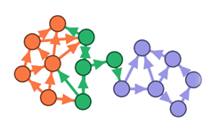
The ExactControllability.m function implements a maximum geometric multiplicity algorithm to identify the number and set of driver nodes in complex network (see included references). Input is an adjacency matrix - directed or undirected.

Please refer to ExactControllability.m for instructions on how to cite.

Cite As

Tapan (2023). Exact controllability of complex networks (https://www.mathworks.com/matlabcentral/fileexchange/49357-exact-controllability-of-complex-networks), MATLAB Central File Exchange. Retrieved June 13, 2023.

  function A = BAgraph_dir(N,mo,m) 
 

  % Generates a scale-free directed adjacency matrix using Barabasi and Albert algorithm 
 

  % Input: N - number of nodes in the network, mo - size of seed, m = average degree. Use mo=m or m<mo. 
 

  % Example: A = BAgraph(300,10,10); 
 

  % Ref: Methods for generating complex networks with selected structural properties for simulations, Pretterjohn et al, Frontiers Comp Neurosci 
 

  % Author: 
 

  % Tapan P Patel, PhD, tapan.p.patel@gmail.com 
 

  % University of Pennsylvania 
 

  hwait = waitbar(0,'Please wait. Generating directed scale-free adjacency matrix'); 
 

  A = zeros(N); 
 

  E = 0; 
 

  for i=1:mo 
 

   for j=i+1:mo 
 

   A(i,j) =1; 
 

   A(j,i) = 1; 
 

   E = E + 2; 
 

end

end

  % Second add remaining nodes with a preferential attachment bias 
 

  for i=mo+1:N 
 

   waitbar(i/N,hwait,sprintf('Please wait. Generating directed scale-free adjacency matrix\n%.1f %%',(i/N)*100)); 
 

   curr_deg =0; 
 

   while(curr_deg<m) 
 

   sample = setdiff(1:N,[i find(A(i,:))]); 
 

   j = datasample(sample,1); 
 

   b = sum(A(j,:))/E; 
 

   r = rand(1); 
 

   if(b>r) 
 

   r = rand(1); 
 

   if(b>r) 
 

   A(i,j) = 1; 
 

   A(j,i) = 1; 
 

   E = E +2; 
 

   else 
 

   A(i,j) = 1; 
 

   E = E +1; 
 

end

   else 
 

   no_connection = 1; 
 

   while(no_connection) 
 

   sample = setdiff(1:N,[i find(A(i,:))]); 
 

   h = datasample(sample,1); 
 

   b = sum(A(h,:))/E; 
 

   r = rand(1); 
 

   if(b>r) 
 

   r = rand(1); 
 

   if(b>r) 
 

   A(h,i) = 1; 
 

   A(i,h) = 1; 
 

   E = E +2; 
 

   else 
 

   A(i,h) = 1; 
 

   E = E+1; 
 

end

   no_connection = 0; 
 

end

end

end

   curr_deg = sum(A(i,:)); 
 

end

end

  delete(hwait); 
 

  %% Controllability of complex networks demo: 
 

  % Examples 1, 2 and 3 are three different network configurations illustrated 
 

  % in Figure 1 of Liu et al, Controllability of complex networks, Nature 
 

  % 2011 
 

  %% Example 1: 
 

  % Directed path, 4 nodes. Node 1 connects to node 2, node 2 connects to 
 

  % node 3, node 3 connects to node 4 
 

clc

  A = [0 1 0 0; 
 

       0 0 1 0; 
 

       0 0 0 1; 
 

       0 0 0 0]; 
 

  [Nd, drivernodes,Nconfig] = ExactControllability(A,'plotting',1) 
 

  % The above command returns Nd = 1, i.e. total of 1 driver node, 
 

  % drivernodes = 1, i.e. node #1 is the driver node 
 

  % Nconfig = 1, i.e. there is only 1 configuration of driver node 
 

  %% Example 2: 
 

  % Directed star. 4 nodes, where node 1 connects to all other 3 nodes. 
 

clc

  A = [0 1 1 1; 
 

      0 0 0 0; 
 

      0 0 0 0; 
 

      0 0 0 0;]; 
 

  [Nd, drivernodes,Nconfig] = ExactControllability(A,'plotting',1) 
 

  % In this example, there are total of 3 driver nodes, Nd = 3. 
 

  % The identity of driver nodes are provided in the vector drivernodes. 
 

  % There are total of 3 distinct configurations of selecting drivernodes, 
 

  % Nconfig = 3. Each time the algorithm is run, a different set of 
 

  % drivernodes will be returned. The possibilites are: {1,3,4}, {1,2,3}, 
 

  % {1,2,4} 
 

  %% Example 3: 
 

clc

  A = [0 1 1 1 1 1; 
 

      0 0 0 0 0 0; 
 

      0 0 0 0 0 0; 
 

      0 0 0 0 0 0; 
 

      0 0 0 0 0 0; 
 

      0 0 0 0 1 0;]; 
 

  [Nd, drivernodes,Nconfig] = ExactControllability(A,'plotting',1) 
 

  % In this example, there are Nd = 4 driver nodes and 4 distinct 
 

  % configurations. The possiblities of drivernodes = {1,2,3,4}, {1,3,4,6}, 
 

  % {1,2,3,6}, {1,2,4,6} 
 

  %% Example 4: 
 

  % Let's try a more complex network. Let's build a scale-free directed 
 

  % network with 300 nodes, using a seed network size of 10 nodes and average 
 

  % connectivity 10. Please see the accompanying BAgraph_dir.m file for more 
 

  % info on the algorithm. The BAgraph_dir algorithm may take some time to 
 

  % generate an adjacency matrix. To save time, you may load a sample 
 

  % adjacency matrix by executing:  
 

  %load('scalefree_adjacency.mat'); 
 

clc

  A = BAgraph_dir(300,10,10); 
 

  % A scale-free network should have a power-law degree distribution. Verify 
 

  % by  
 

  figure; hist(sum(A),20); xlabel('Degree'); ylabel('Count'); 
 

  [Nd, drivernodes,Nconfig] = ExactControllability(A,'plotting',1) 
 

  % There are Nd = 33 driver nodes and only 1 configuration. The identity of 
 

  % driver nodes is provided in the variable drivernodes. 
 

  % You will note that the drivernodes have very low in-degrees 
 

  % sum(A(:,drivernodes) 
 

  %% Example 5: 
 

  % Lastly, let's try a random undirected symmetric Erdos Reyni network of 300 nodes with 0.01 
 

  % probability of connection between any pair-wise nodes 
 

clc

  A = erdos_reyni(300,0.01); 
 

  [Nd, drivernodes,Nconfig] = ExactControllability(full(A),'plotting',1) 
 

  % There are Nd = 22 driver nodes and 16 different ways to choose 22 driver 
 

  % nodes. Note: as the network becomes less sparse, i.e. as the probability 
 

% of connection incresease from 0.01, the number of driver nodes decreases.

   function A=erdos_reyni(n,p)  
  
   % ERDOS_REYNI Generates a random Erdos-Reyni (Gnp) graph  
  
   %  
  
   % A=erdos_reyni(n,p) generates a random Gnp graph with n vertices and where  
  
   % the probability of each edge is p.  The resulting graph is symmetric.  
  
   %  
  
   % Example:  
  
   %   A = erdos_reyni(100,0.05);  
  
   A = triu(rand(n)<p,1);  
  
   A = sparse(A);  
  
   A = A+A';  
  
   function [Nd,drivernodes,Nconfigs,ld,C] = ExactControllability(A,varargin)  
  
   % Computes the exact controllability of matrix A of arbitrary structure.   
  
   % Input: adjacency matrix A, where entry in row i, column j, indicates a  
  
   % connection from i to j.   
  
   % Use second argument (..,'plotting',0) to disable generating network figure.  
  
   % Default is to plot.  
  
   % Returns Nd = number of driver nodes, drivernodes = list of driver node IDs,   
  
   % Nconfigs = number of different configurations that satisfy the requirement of Nd.   
  
   % Each time the code is run, a different set of configuration of driver nodes   
  
   % will be returned. The total number of driver nodes (Nd) remains constant.  
  
   % Ref: Exact Controllability of complex networks by Yuan et al, Nat Comm 2013  
  
   % Code written by:  
  
   % Tapan P Patel, PhD, tapan.p.patel@gmail.com  
  
   % University of Pennsylvania  
  
   % Please cite: Patel TP et al, Automated quantification of neuronal   
  
   % networks and single-cell calcium dynamics using calcium imaging.  
  
   % J Neurosci Methods, 2015.  
  
   % Please see the demo.m file for examples.  
  
   % Examples 1, 2 and 3 are three different network configurations illustrated  
  
   % in Figure 1 of Liu et al, Controllability of complex networks, Nature  
  
   % 2011  
  
   % Example 1:  
  
   % Directed path, 4 nodes. Node 1 connects to node 2, node 2 connects to  
  
   % node 3, node 3 connects to node 4  
  
   % A = [0 1 0 0;  
  
   %      0 0 1 0;  
  
   %      0 0 0 1;  
  
   %      0 0 0 0];  
  
   % [Nd, drivernodes,Nconfig] = ExactControllability(A,'plotting',1);  
  
   % The above command returns Nd = 1, i.e. total of 1 driver node,  
  
   % drivernodes = 1, i.e. node #1 is the driver node  
  
   % Nconfig = 1, i.e. there is only 1 configuration of driver node  
  
   % Example 2:  
  
   % Directed star. 4 nodes, where node 1 connects to all other 3 nodes.  
  
   % A = [0 1 1 1;  
  
   %     0 0 0 0;  
  
   %     0 0 0 0;  
  
   %     0 0 0 0;];  
  
   % [Nd, drivernodes,Nconfig] = ExactControllability(A,'plotting',1);  
  
   % In this example, there are total of 3 driver nodes, Nd = 3.  
  
   % The identity of driver nodes are provided in the vector drivernodes.  
  
   % There are total of 3 distinct configurations of selecting drivernodes,  
  
   % Nconfig = 3. Each time the algorithm is run, a different set of  
  
   % drivernodes will be returned. The possibilites are: {1,3,4}, {1,2,3},  
  
   % {1,2,4}  
  
   % Example 3:  
  
   % A = [0 1 1 1 1 1;  
  
   %     0 0 0 0 0 0;  
  
   %     0 0 0 0 0 0;  
  
   %     0 0 0 0 0 0;  
  
   %     0 0 0 0 0 0;  
  
   %     0 0 0 0 1 0;];  
  
   % [Nd, drivernodes,Nconfig] = ExactControllability(A,'plotting',1);  
  
   % In this example, there are Nd = 4 driver nodes and 4 distinct  
  
   % configurations. The possiblities of drivernodes = {1,2,3,4}, {1,3,4,6},  
  
   % {1,2,3,6}, {1,2,4,6}  
  
   % Example 4:  
  
   % Let's try a more complex network. Let's build a scale-free directed  
  
   % network with 300 nodes, using a seed network size of 10 nodes and average  
  
   % connectivity 10. Please see the accompanying BAgraph_dir.m file for more  
  
   % info on the algorithm. The BAgraph_dir algorithm may take some time to  
  
   % generate an adjacency matrix. To save time, you may load a sample  
  
   % adjacency matrix by executing: load('scalefree_adjacency.mat');  
  
   % A = BAgraph_dir(300,10,10);  
  
   % A scale-free network should have a power-law degree distribution. Verify  
  
   % by   
  
   % figure; hist(sum(A),20); xlabel('Degree'); ylabel('Count');  
  
   % [Nd, drivernodes,Nconfig] = ExactControllability(A,'plotting',1);  
  
   % There are Nd = 33 driver nodes and only 1 configuration. The identity of  
  
   % driver nodes is provided in the variable drivernodes.  
  
   % You will note that the drivernodes have very low in-degrees  
  
   % sum(A(:,drivernodes)  
  
   % Example 5:  
  
   % Lastly, let's try a random undirected symmetric Erdos Reyni network of 300 nodes with 0.01  
  
   % probability of connection between any pair-wise nodes  
  
   % A = erdos_reyni(300,0.01);  
  
   % [Nd, drivernodes,Nconfig] = ExactControllability(full(A),'plotting',1);  
  
   % There are Nd = 22 driver nodes and 16 different ways to choose 22 driver  
  
   % nodes. Note: as the network becomes less sparse, i.e. as the probability  
  
   % of connection incresease from 0.01, the number of driver nodes decreases.  
  
   %%  
  
   % In Yuan's algorithm, a(i,j) refers to a connection from j to i rather than   
  
   % a connection from i to j. So the input needs to be transposed.  
  
   % Multiplicity of an eigenvalue i is the number of times lambda_i is repeated   
  
   % (tolerance 1e-8). lambda_i that corresponds to the maximum multiplicity is   
  
   % then used to compute a geomtric multiplicity.  
  
   % C is the column reduced matrix whose dependent rows  are the identities of   
  
   % the driver nodes. There can be more than 1 set of driver nodes consistent   
  
   % with the requirement N_D total driver nodes.  
  
   plotting = 1;  
  
   % ------------------------------------------------------------------------------  
  
   % parse varargin  
  
   % ------------------------------------------------------------------------------  
  
   if nargin > 2  
  
       for i = 1:2:length(varargin)-1  
  
           if isnumeric(varargin{i+1})  
  
               eval([varargin{i} '= [' num2str(varargin{i+1}) '];']);  
  
           else  
  
               eval([varargin{i} '=' char(39) varargin{i+1} char(39) ';']);  
  
           end  
  
       end  
  
   end  
  
   A = double(A);  
  
   A = A';  
  
   lambda = eig(A);  
  
   multiplicity = -1;  
  
   lambda_M = 0;  
  
   for i=1:length(lambda)  
  
    x = length(find(abs(lambda(i)-lambda)<1e-8));  
  
    if(~isempty(x) && x>multiplicity)  
  
    multiplicity = x;  
  
    lambda_M = lambda(i);  
  
    end  
  
   end  
  
   N = size(A,1);  
  
   mu_M = N - rank(lambda_M*eye(N)-A);  
  
   Nd = mu_M;  
  
   %%  
  
   % mu_M is the number of minimum driver nodes  
  
   % lambda_M is used to identify the set of driver nodes  
  
   M = A- lambda_M*eye(N);  
  
   C = rref(M')';  
  
   % Linearly dependent rows of C are the driver nodes. However, there can be more than 1 configuration of the set of driver nodes. Let's enumerate the possibilities. Row i is linearly independent if C(i,i) ~=0 and all other entries in that row are 0. Similarly row i is linearly dependent if either all rows are 0 or there are more than 1 nonzero entries in the row. Configurations of driver nodes would include all the dependent rows and a node from each of the independent row if the multiplicity at row i is >1.  
  
   li = cell(N,1);  
  
   ld = [];  
  
   for i=1:N  
  
    if(nnz(C(i,:))==1)  
  
    idx = find(C(i,:));  
  
    x = li{idx};  
  
    x = [x i];  
  
    li{idx} = x;  
  
    else  
  
    ld = [ld i];  
  
    end  
  
   end   
  
   % Driver node configurations:  
  
   DriverConfigs = cell(N,1);  
  
   Nconfigs = 1;  
  
   for i=1:N  
  
    if(length(li{i})>1)  
  
    % Keep 1 and the rest are dependent rows which make them drivers  
  
    idx = li{i};  
  
    DriverConfigs(i) = {nchoosek(idx,length(idx)-1)};  
  
    % Number of possible configurations is the product of the size of each DriverConfigs{i}  
  
    Nconfigs = Nconfigs*size(DriverConfigs{i},1);  
  
    end  
  
   end  
  
   % Give a permutation of driver node configuration.  
  
   drivernodes = ld;  
  
   for i=1:N  
  
    if(~isempty(DriverConfigs{i}))  
  
    x = DriverConfigs{i};  
  
    k = randsample(size(x,1),1);  
  
    drivernodes = [drivernodes x(k,:)];  
  
    end  
  
   end  
  
   if(isempty(drivernodes))  
  
       drivernodes = 0;  
  
       Nd = 0;  
  
       Nconfigs = 0;  
  
   end  
  
   %% Plot  
  
   if(plotting)  
  
   xy = rand(size(A,1),2);  
  
   gplotdc(A,xy);  
  
   % Color driver nodes in blue  
  
   hold on  
  
   plot(xy(drivernodes,1),xy(drivernodes,2),'ro','MarkerFaceColor','r','MarkerSize',6);  
  
   title(sprintf('%d driver nodes identified\nNodes in red are driver nodes.',Nd));  
  
   end

  function gplotdc(A,xy,varargin) 
 

  %GPLOTDC Plot a Directed Graph 
 

  % GPLOTDC(A,XY) Plots the Directed Graph represented by adjacency 
 

  %   matrix A and points xy using the default style described below 
 

  % GPLOTDC(A,XY,PARAM1,VAL1,PARAM2,VAL2,...) Plots the Directed Graph 
 

  %   using valid parameter name/value pairs 
 

%

  %   Inputs: 
 

  %       A     - NxN adjacency matrix, where A(I,J) is nonzero (=1) 
 

  %               if and only if there is an edge between points I and J 
 

  %       xy    - Nx2 matrix of x/y coordinates 
 

  %       ...   - Parameter name/value pairs that are consistent with 
 

  %               valid PLOT parameters can also be specified 
 

%

  %   Default Plot Style Details: 
 

  %       1. Undirected (2-way) edges are plotted as straight solid lines 
 

  %       2. Directed (1-way) edges are plotted as curved dotted lines with 
 

  %           the curvature bending counterclockwise moving away from a point 
 

  %       3. Any vertex that is connected to itself is plotted with a 
 

  %           circle around it 
 

%

  %   Example: 
 

  %       % plot a directed graph using default line styles 
 

  %       n = 9; t = 2*pi/n*(0:n-1); 
 

  %       A = round(rand(n)); 
 

  %       xy = [cos(t); sin(t)]'; 
 

  %       gplotdc(A,xy); 
 

  %       for k = 1:n 
 

  %           text(xy(k,1),xy(k,2),['  ' num2str(k)],'Color','k', ... 
 

  %               'FontSize',12,'FontWeight','b') 
 

  %       end 
 

%

  %   Example: 
 

  %       % plot a directed graph using plot name/value parameter pairs 
 

  %       n = 9; t = 2*pi/n*(0:n-1); 
 

  %       A = round(rand(n)); 
 

  %       xy = [cos(t); sin(t)]'; 
 

  %       gplotdc(A,xy,'LineWidth',2,'MarkerSize',8); 
 

%

  %   Example: 
 

  %       % plot a directed graph using a different color and linestyle 
 

  %       n = 9; t = 2*pi/n*(0:n-1); 
 

  %       A = round(rand(n)); 
 

  %       xy = [cos(t); sin(t)]'; 
 

  %       gplotdc(A,xy,'Color',[0.67 0 1],'LineStyle',':'); 
 

%

  % See also: gplot, plot 
 

%

  % Author: Joseph Kirk 
 

  % Email: jdkirk630@gmail.com 
 

  % Release: 1.0 
 

  % Release Date: 4/12/08 
 

  % Process Inputs 
 

  if nargin < 2 
 

      error('Not enough input arguments.'); 
 

end

  [nr,nc] = size(A); 
 

  [n,dim] = size(xy); 
 

  if (~n) || (nr ~= n) || (nc ~= n) || (dim < 2) 
 

      eval(['help ' mfilename]); 
 

      error('Invalid input. See help notes above.'); 
 

end

  params = struct(); 
 

  for var = 1:2:length(varargin)-1 
 

      params.(varargin{var}) = varargin{var+1}; 
 

end

  % Parse the Adjacency Matrix 
 

  A = double(logical(A)); 
 

  iA = diag(diag(A));         % self-connecting edges 
 

  dA = A.*(1-A');             % directed edges (1-way) 
 

  uA = A-dA-iA;               % undirected edges (2-way) 
 

  % Make NaN-Separated XY Vectors 
 

  [ix,iy] = makeXY(iA,xy); 
 

  [dx,dy] = makeXY(dA,xy); 
 

  [ux,uy] = makeXY(tril(uA,0),xy); 
 

  % Add Curvature to Directed Edges 
 

  dX = dx; 
 

  dY = dy; 
 

  pct = 0.04; 
 

  for k = 1:4 
 

      [dX,dY,pct] = makeCurved(dX,dY,pct); 
 

end

  % Plot the Graph 
 

  plot(ux,uy,'b-',params) 
 

  hold on 
 

  plot(dX,dY,'r--',params) 
 

  plot(ix,iy,'ko',params) 
 

  plot(xy(:,1),xy(:,2),'k.') 
 

  hold off 
 

      function [x,y] = makeXY(A,xy) 
 

          if any(A(:)) 
 

              [J,I] = find(A'); 
 

              m = length(I); 
 

              xmat = [xy(I,1) xy(J,1) NaN(m,1)]'; 
 

              ymat = [xy(I,2) xy(J,2) NaN(m,1)]'; 
 

              x = xmat(:); 
 

              y = ymat(:); 
 

          else 
 

              x = NaN; 
 

              y = NaN; 
 

end

end

      function [X,Y,PCT] = makeCurved(x,y,pct) 
 

          N = length(x); 
 

          if N < 2 
 

              X = x; 
 

              Y = y; 
 

          else 
 

              M = 2*N-1; 
 

              X = zeros(1,M); 
 

              Y = zeros(1,M); 
 

              X(1:2:M) = x; 
 

              Y(1:2:M) = y; 
 

              X(2:2:M-1) = 0.5*(x(1:N-1)+x(2:N))+pct*diff(y); 
 

              Y(2:2:M-1) = 0.5*(y(1:N-1)+y(2:N))-pct*diff(x); 
 

end

          PCT = 0.5*pct; 
 

end

end

【关闭】